Identify heart sound using 2D convolutional neural network model (2D CNN)

Youtube Link for system demo

https://www.youtube.com/watch?v=KOdiLGD8BZc&t=2s

Sound Identification

Listen to understand the prospect of human-like sound or the sound present in the natural environment can be performed by machines with the use of AI techniques. Supervised learning is one of the AI techniques that is commonly applied in classification and regression. In the classification and regression process, a model is built before training and learning from a huge amount of labeled training datasets which can either consist of the feature vector that describes the object of the event or the ground-truth output represented by the label.

Signal processing has been deployed in the medical field for the diagnosis process to achieve a more accurate and informative result from the system. The bio-signals such as the electrocardiogram (ECG) or phonocardiogram (PCG) do provide the signal features that can be extracted and fed into machine learning or supervised learning algorithms to classify heart valve diseases. The signal features that vary with respect to the time domain, amplitude domain, frequency content, and intensity can be used to differentiate between normal and abnormal heart sound.

Automated heart sound classification with machine learning is generally to improve the adaptation of the algorithm of the machine learning model to the changes of the heart sounds like the heart sound from the recorded audio data is very subtle. To improve the accuracy of classification, some fundamental procedures or techniques used in signal processing need to be taken into account. The procedures of heart sound classification using a machine learning model are described in the following sections.

Denoising / Cleaning

Fast Fourier transform (FFT) is calculated over the noise audio clip and signal audio clip to transform the signal into its frequency domain. The mask is then smoothed with a filter over frequency and time before applying it to the FFT of the signal audio clip.

import noisereduce as nr
#remove the noise of the signal
reduced_noise = nr.reduce_noise(audio_clip=signal,noise_clip=signal, verbose=False)
#change the output to ndarray
reduced_signal_noise = np.array(reduced_noise)
np.set_printoptions(threshold=np.inf)

Normalization

The de-noised signal is then normalized with the maximum value of the signal as shown below,

import numpy as np
#extract the maximum signal
maximum_signal = max(np.abs(reduced_signal_noise))
#normalize the signal
normalized_signal = np.array([(abs(signal) / maximum_signal) for signal in reduced_signal_noise])

Segmentation

In the segmentation process, Shannon energy is then calculated over the normalized signal. This energy is a square of the input signal because the square of signal is proximity to signal energy.

#iterate through the normalized signal
for x in range(0, len(normalized_signal)):
    #power the signal by 2 
    signal_sample = abs(normalized_signal[x]) ** 2 
    if signal_sample <= 0: #set the signal to 1 if it is empty
       signal_sample = 1.0
    
    #calculate Shannon energy
    shannon_energy = signal_sample * math.log(signal_sample)
    
    #replace the normalized signal with Shannon energy       
    normalized_signal[x] = shannon_energy

After this, the vector of Shannon energies is then passed for averaging. Shannon energies are averaged in continuous signals with 0.01 seconds intervals.

import numpy as np
#obtain the length of signal
length_of_signal = len(shannon_energy_signal)
#Initialize the signal
segment_signal = 0 
#Set the segmented signal to 0.0002 seconds for realtime analysis, otherwise 0.02 seconds for audio recorder
if realtime:
   #set the segment of 0.0002 seconds
   segment_signal = int(sample_rate * 0.0002)
else:
   #set the segment of 0.02 seconds
   segment_signal = int(sample_rate * 0.02)
segment_energy = [] #initialize the array
for x in range(0, len(shannon_energy_signal), segment_signal):
    sum_signal = 0 
    #retrieve the signal in a segment of 0.02 seconds
    current_segment_energy=shannon_energy_signal[x:x+segment_signal]
    for i in range(0, len(current_segment_energy)):
        #sum up the Shannon energy
        sum_signal += current_segment_energy[i]
    #assign the average Shannon energy to array    
    segment_energy.append(-(sum_signal/segment_signal))
#convert to numpy array
segment_energy_signal = np.array(segment_energy)

The average Shannon energy is then normalized to convert into an energy package, which is also known as the Shannon energy envelope using the mean and the standard deviation. The envelope decreases the signal base and places the signal below the baseline.

import numpy as np
import librosa, librosa.display
#calculate mean
mean_SE = np.mean(segment_energy_signal)
#calculate standard deviation
std_SE = np.std(segment_energy_signal)
#calculate Shannon Envelope
for x in range(0, len(segment_energy_signal)):
    envelope = 0
    envelope = (segment_energy_signal[x] - mean_SE) / std_SE
    segment_energy_signal[x] = envelope
shannon_envelope = segment_energy_signal
#calculate envelope size
envelope_size = range(0, shannon_envelope.size)
#calculate envelope time
envelope_time = librosa.frames_to_time(envelope_size,hop_length=442)

A threshold value is a definition to determine peaks (QRS complex location) with the fact that the sample with greater amplitude than the threshold is chosen as output. The threshold value is defined using the mean, standard deviation, and a constant.

import numpy as np
segment_signal = [0] * len(clean_signal)
threshold = 0
k = 0.001
#calculate threshold
if std_SE < mean_SE:
   threshold = abs(k * mean_SE * (1 - std_SE ** 2))
elif std_SE > mean_SE:
     threshold = abs(k * std_SE * (1 -  mean_SE ** 2))
#extract the signal that is greater than threshold   
for x in range(0, len(clean_signal)):
    if np.abs(clean_signal[x]) > threshold:
       segment_signal[x] = clean_signal[x]
segmented_signal = np.array(segment_signal)
#remove 0 
clean_segmented_signal = np.delete(segmented_signal, np.where(segmented_signal == 0))

Feature Extraction

A total of seven features are extracted from different domains. The features are processed using “librosa” and “pyAudioAnalysis” libraries. The extracted features included zero-crossing rate, Mel-frequency cepstral coefficients (MFCCs), spectral centroid, spectral roll-off, spectral flux, frequency, and energy entropy. The zero-crossing rate and the energy entropy are the time domain features, whereas the other five features belong to the frequency domain features.

Zero-crossing rate

from pyAudioAnalysis import ShortTermFeatures as stf
zero_crossing_rate = stf.zero_crossing_rate(clean_segmented_signal)

Mel-frequency cepstral coefficients (MFCCs)

import librosa, librosa.display
import numpy as np
mfcc =librosa.feature.mfcc(clean_segmented_signal.astype('float32'), sr=sample_rate)
mean_mfcc = np.mean(mfcc)
std_mfcc = np.std(mfcc)

Spectral centroid

import librosa, librosa.display
spectral_centroid = librosa.feature.spectral_centroid(clean_segmented_signal, sr=sample_rate)

Spectral roll-off

import librosa, librosa.display
spectral_rolloff = librosa.feature.spectral_rolloff(clean_segmented_signal, sr=sample_rate)

Spectral flux

from pyAudioAnalysis import ShortTermFeatures as stf
import numpy as np
#divide the segmented signal length by half
fft_frame_length = len(clean_segmented_signal) / 2
#extract the signal by half
first_frame = clean_segmented_signal[:int(fft_frame_length)]
second_frame = clean_segmented_signal[int(fft_frame_length):]
frame_step = 1
while(first_frame.shape != second_frame.shape):
      first_frame = clean_segmented_signal[:frame_step+int(fft_frame_length)]
      second_frame = clean_segmented_signal[int(fft_frame_length):]
            frame_step = frame_step + 1
#calculate the fft of the signal
fft_first_frame = np.array([np.fft.fft(first_frame)])
fft_second_frame = np.array([np.fft.fft(second_frame)])
#extract the spectral flux features
spectral_flux = np.array(stf.spectral_flux(np.abs(fft_first_frame), np.abs(fft_second_frame)))

Frequency

import numpy as np
frequency_domain = np.array([np.fft.fft(clean_segmented_signal)])
#calculate mean
mean_frequency_domain = np.mean(frequency_domain)
#calculate standard deviation
std_frequency_domain = np.std(frequency_domain)
#extract the real and the imaginary number from complex number
mean_frequency_domain_real = mean_frequency_domain.real
mean_frequency_domain_imaginary = mean_frequency_domain.imag

Energy entropy

from pyAudioAnalysis import ShortTermFeatures as stf
import numpy as np
#Extract the energy entropy
energy_entropy = np.array(stf.energy_entropy(clean_segmented_signal))

The features are used as the characteristics of each sample of the heart sound. The values are then saved in a comma-separated value (CSV) file according to the respective column. Indeed, a new column is added to label the types of heart sounds. For instance, 1 represents normal heart sound, 2 represents murmur heart sound, 3 represents extrasystole heart sound, and 4 represents extra heart sound respectively.

2D Convolutional Neural Network (CNN) Model

The structure of the 2D CNN model resembles a multi-layer perceptron (MLP) and each neuron in the MLP is associated with an activation function that maps the weighted inputs to the output. There are some basic layers in CNN model, which are convolutional layer, max-pooling layer, dropout, batch normalization, and a fully connected layer or a dense layer, with a rectified linear activation function in CNN architecture. In addition, the design of the structure of the model is shown below,

Model Summary

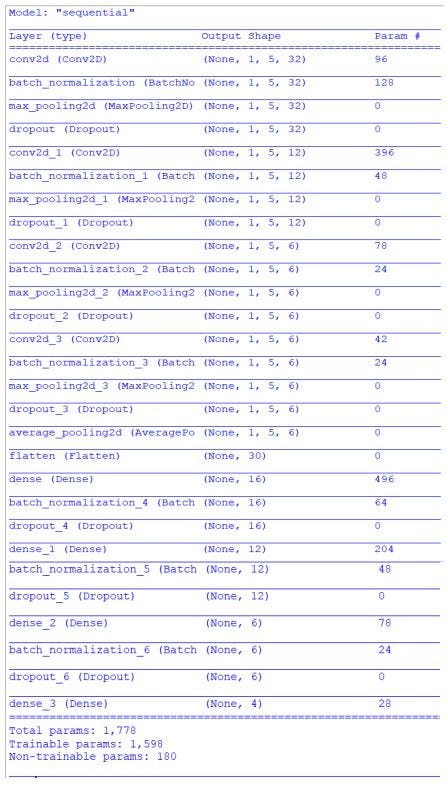
The proposed two-dimensional (2D) convolutional neural network (CNN) model is trained and tested using the datasets saved in the CSV file. The dataset is then split into 80% of the training set, 10% of the validation set, and 10% of the testing set.

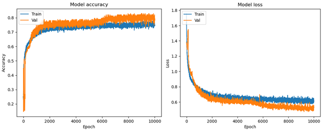
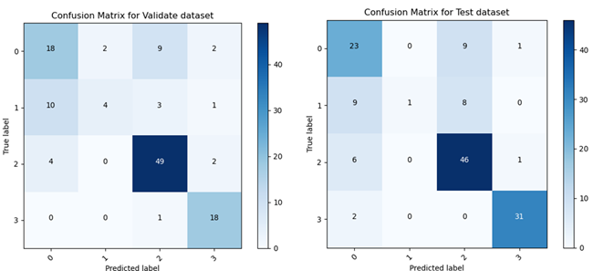
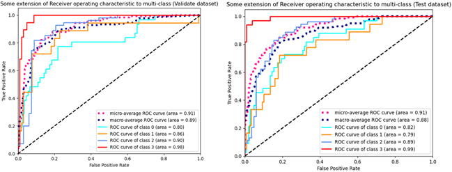
Results

Performance Graphs

Confusion Matrix

Receiver Operating Characteristic (ROC) curve

Reference

Beyramienanlou H, Lotfivand N (2017) Shannon’s energy-based algorithm in ECG signal processing. Computational and mathematical methods in medicine 2017:1–16. https://doi.org/10.1155/2017/8081361